In the previous article I wrote about one way to efficiently represent graphs on GPUs for GNNs, by essentially keeping everything in tensors and accessing them via sparse matrix indices (I suggest checking it out before reading this). In this one, I'll show how that representation lets us fuse the graph attention computation in RTMScore into a single Triton kernel, achieving a 4x speedup over PyTorch at batch size 64.
Background
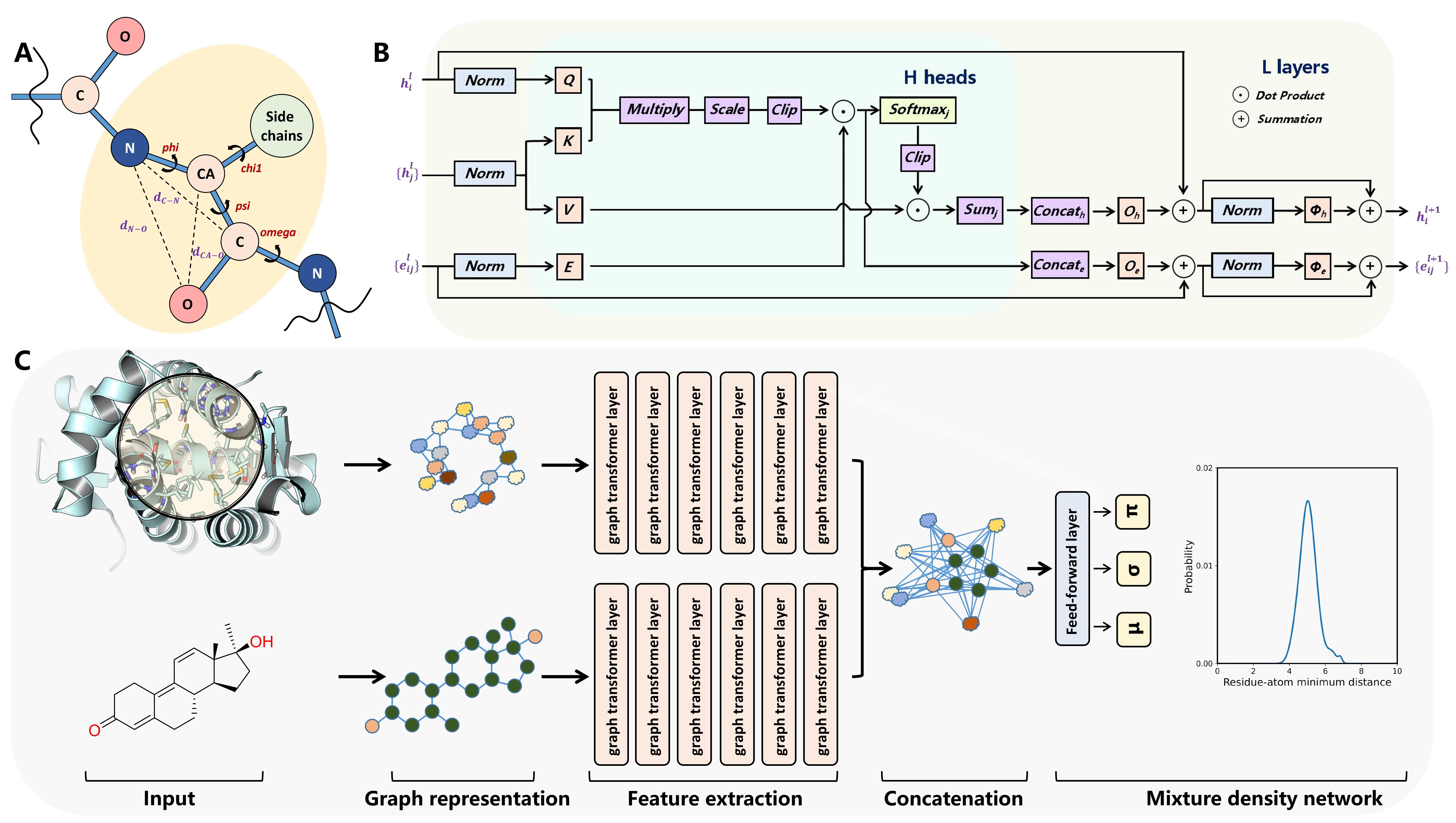
Graph attention in RTMScore (and other similar graph transformers) works like this:
- For each node, compute the \(Q\), \(K\) and \(V\) projections.
- For each edge, compute the \(E\) projection.
- For each node \(h_i\) and its incoming neighbours \(\{h_j\}\), perform attention by:
- Computing the element-wise product \(q_i \odot k_j \odot e_{ij}\), where \(e_{ij}\) is the \(E\) projection of the edge from \(j\) to \(i\). I'm leaving out some scaling and clipping for now; we'll see the exact order in the code.
- Summing over the feature dimension to get a scalar logit \(\ell_{ij}\) for each head, then clipping it to \([-5, 5]\) before exponentiating: \(s_{ij} = \exp(\operatorname{clip}(\ell_{ij}, -5, 5))\).
- Normalizing over incoming edges to get the attention weights \(\alpha_{ij} = s_{ij} / (\sum_k s_{ik} + \epsilon)\). This is the softmax, with a small epsilon in the denominator.
- Computing the final attention vector as the weighted sum of the value vectors: \(o_i = \sum_j \alpha_{ij} v_j\).
The attention layers have multiple heads, so the final vectors get concatenated and projected by the \(O\) matrix. One peculiarity of RTMScore is that the edge projection scales the element-wise query/key product,
and the resulting vector is also used to update the edge features before being reduced to a scalar logit. These things don't change the overall approach to the kernel much.
What we are effectively doing is computing a score (and a corresponding scaled value vector) for each edge in the graph, and then "selectively" summing them based on the destination
node. This selective reduction is a scatter add on the destination index. In the PyTorch examples below, I use index_add_ to perform this scatter add: it takes a 1D destination index and adds each edge's values to the corresponding node.
# we first build a zero tensor to use as an accumulator for the scatter add
attn_result = v_scaled.new_zeros((N_NODES, ATTN_DIM)).index_add_(0, coo_col_index, v_scaled) # (N_NODES, ATTN_DIM)
And here the problems start. If you don't know, some versions of TensorRT simply do not support a scatter with a reduce sum. Because I was (and am) working on a TensorRT backend for this model, it meant that I had to implement the kernel myself and wrap it in a TensorRT plugin. The original intention was to just write the scatter add (fused with a normalization step which I'll show later), but then I noticed that the same approach could quite easily be used for the whole attention computation, so I thought: why not just fuse everything?
Optimizing the scatter add in Triton
The reference scatter add implementation is this. All PyTorch timings in this article use eager mode.
def reference_scatter_add(
    v_scaled: torch.Tensor,
    score: torch.Tensor,
    destination_indices: torch.Tensor,
    num_nodes: int,
) -> torch.Tensor:
    numerator = torch.zeros(
        num_nodes,
        v_scaled.shape[1],
        v_scaled.shape[2],
        dtype=v_scaled.dtype,
        device=v_scaled.device,
    ).index_add_(0, destination_indices, v_scaled)
    denominator = torch.zeros(
        num_nodes,
        score.shape[1],
        1,
        dtype=score.dtype,
        device=score.device,
    ).index_add_(0, destination_indices, score)
    return numerator / (denominator + EPSILON)
Note that here we are actually performing two scatters, as we are also normalizing the final vector by the sum of the scores (the denominator of the softmax, which is deferred to the end). As you can see,
both scatters process the same edges, with one value vector and one score per head for each edge, and use the same destination index. This makes the two scatters and the final normalization easy to fuse.
My first approach was to just assign one program to each node, make it iterate over the v_scaled and score tensors, masking out non-relevant edges using the destination_indices index. Additionally, instead of
processing each edge one by one, we process them in groups. This is a gather approach: each program computes the full output of a single node, so there are no atomic operations.
@triton.jit
def scat_add_kernel_gather(v_scaled_ptr, score_ptr, destination_indices_ptr, num_nodes, num_edges, out_ptr, epsilon, NUM_HEADS: tl.constexpr, HEAD_DIM: tl.constexpr, BLOCK_SIZE: tl.constexpr):
    pid_0 = tl.program_id(0) # one block per node
    # accumulator for the v_scaled vectors
    out = tl.zeros((NUM_HEADS, HEAD_DIM), tl.float32)
    n_heads_dim_offsets = tl.arange(0, NUM_HEADS)
    head_dim_offsets = tl.arange(0, HEAD_DIM)
    out_offsets = pid_0 * NUM_HEADS * HEAD_DIM + n_heads_dim_offsets[:, None] * HEAD_DIM + head_dim_offsets[None, :]
    # accumulator for the scores
    z = tl.zeros((NUM_HEADS,1), tl.float32)
    # process edges in BLOCK_SIZE blocks
    for i in range(0, num_edges, BLOCK_SIZE):
        edge_offsets = i + tl.arange(0, BLOCK_SIZE)
        edge_mask = edge_offsets < num_edges
        dst_indices = tl.load(
            destination_indices_ptr + edge_offsets, mask=edge_mask, other=-1
        )
        # load only v_scaled/scores of incoming edges
        dst_mask = dst_indices == pid_0
        v_scaled_offsets = edge_offsets[:, None, None] * NUM_HEADS * HEAD_DIM + n_heads_dim_offsets[None, :, None] * HEAD_DIM + head_dim_offsets[None, None, :]
        v_scaled_mask = edge_mask[:, None, None] & dst_mask[:, None, None]
        # (BLOCK_SIZE, NUM_HEADS, HEAD_DIM)
        v_scaled = tl.load(v_scaled_ptr + v_scaled_offsets, mask=v_scaled_mask, other=0.0)

        score_offsets = edge_offsets[:, None, None] * NUM_HEADS * 1 + n_heads_dim_offsets[None, :, None] * 1 + tl.arange(0, 1)[None, None, :]
        score_mask = edge_mask[:, None, None] & dst_mask[:, None, None]
        # (BLOCK_SIZE, NUM_HEADS, 1)
        score = tl.load(score_ptr + score_offsets, mask=score_mask, other=0.0)

        # we reduce over the edge_offsets axis
        out += tl.sum(v_scaled, axis=0)
        z += tl.sum(score, axis=0)

    # final normalization
    out = out / (z + epsilon)
    tl.store(out_ptr + out_offsets, out)
The results, however, are pretty underwhelming.
| Batch size | PyTorch | Triton |
|---|---|---|
| 1 | 8.882 | 2.271 |
| 16 | 13.135 | 111.059 |
| 32 | 17.027 | 294.819 |
| 64 | 28.890 | 1094.823 |
While at BS=1 the kernel beats the baseline, with larger batches it performs worse. By a lot.
Profiling it with ncu doesn't immediately help. The overall compute and memory throughputs shown on the NVIDIA Nsight Compute summary page are both around 73%, which I'll use throughout this article. Nsight Compute reports
some problems with the "L1TEX Global Load Access Pattern", as on average only 50% of the bytes in each loaded sector are used. Fixing this access pattern would give
an estimated 35% speedup, which definitely doesn't fix the roughly 38x slowdown at BS=64.
The real culprit lies in the huge amount of unnecessary work that the kernel is doing. Let's say that each graph is made of 100 nodes, and on average each node is connected to 10 other nodes.
This means that, for each node, only 10 edges' v_scaled vectors and score values will actually be useful, while the others will be set to 0 by the masked load. But we are still doing the two sum-reductions and
accumulations even if we haven't actually loaded anything useful! At BS=1, we have \(10\) useful edges out of \(10 \cdot 100 = 1000\), so \(99\%\) of the edge slots being reduced are irrelevant to that node. At BS=64,
we still have only \(10\) useful edges, but now the total is \(64000\)! Most value and score loads are masked out, but the reductions still process those slots, and every program still loads the full destination index.
We are keeping the GPU busy with a lot of work that doesn't contribute to the output.
Therefore, we can improve the kernel by skipping iterations which do not contain any relevant edges. After computing dst_mask, we can check whether any element is 1 with an or-reduction.
@triton.jit
def scat_add_kernel_gather_skip(v_scaled_ptr, score_ptr, destination_indices_ptr, num_nodes, num_edges, out_ptr, epsilon, NUM_HEADS: tl.constexpr, HEAD_DIM: tl.constexpr, BLOCK_SIZE: tl.constexpr):
    pid_0 = tl.program_id(0) # one block per node
    out = tl.zeros((NUM_HEADS, HEAD_DIM), tl.float32)
    n_heads_dim_offsets = tl.arange(0, NUM_HEADS)
    head_dim_offsets = tl.arange(0, HEAD_DIM)
    out_offsets = pid_0 * NUM_HEADS * HEAD_DIM + n_heads_dim_offsets[:, None] * HEAD_DIM + head_dim_offsets[None, :]
    z = tl.zeros((NUM_HEADS,1), tl.float32)
    for i in range(0, num_edges, BLOCK_SIZE):
        edge_offsets = i + tl.arange(0, BLOCK_SIZE)
        edge_mask = edge_offsets < num_edges
        dst_indices = tl.load(
            destination_indices_ptr + edge_offsets, mask=edge_mask, other=-1
        )
        dst_mask = dst_indices == pid_0
        # v_scaled/score load, reduction and accumulation is done only
        # if there's at least one incoming edge
        if tl.reduce_or(dst_mask, axis=None):
            v_scaled_offsets = edge_offsets[:, None, None] * NUM_HEADS * HEAD_DIM + n_heads_dim_offsets[None, :, None] * HEAD_DIM + head_dim_offsets[None, None, :]
            v_scaled_mask = edge_mask[:, None, None] & dst_mask[:, None, None]
            v_scaled = tl.load(v_scaled_ptr + v_scaled_offsets, mask=v_scaled_mask, other=0.0)

            score_offsets = edge_offsets[:, None, None] * NUM_HEADS * 1 + n_heads_dim_offsets[None, :, None] * 1 + tl.arange(0, 1)[None, None, :]
            score_mask = edge_mask[:, None, None] & dst_mask[:, None, None]
            score = tl.load(score_ptr + score_offsets, mask=score_mask, other=0.0)

            out += tl.sum(v_scaled, axis=0)
            z += tl.sum(score, axis=0)

    out = out / (z + epsilon)
    tl.store(out_ptr + out_offsets, out)
The results are much better now.
| Batch size | PyTorch | Triton | Triton + skip |
|---|---|---|---|
| 1 | 8.882 | 2.271 | 2.524 |
| 16 | 13.135 | 111.059 | 15.950 |
| 32 | 17.027 | 294.819 | 34.366 |
| 64 | 28.890 | 1094.823 | 82.916 |
The optimization also shows up in the profiler. At BS=64, the number of scheduled warp instructions drops from 258.07 M
to 14.25 M. We have removed about 94% of the instructions by skipping work on unrelated, masked edges!
However, there are still problems. At BS=64, the kernel is still about 2.9x slower than the baseline. The profiler now shows pretty bad throughput stats (compute at 46% and memory at 39%).
The diagnostics also don't really help, as they are similar to the previous case. At this point I tried a few different things such as:
- Keeping the accumulators with the
BLOCK_SIZEleading dimension and reducing only at the end. This, however, kills occupancy, as the storage required by each block increases significantly. - Assigning a separate program to each node/head pair.
- Making each program compute multiple nodes.
None of these experiments worked out, because none of them tackle the actual issue with this approach. While we are skipping the computations for unrelated edges, we are still iterating through them and
loading dst_indices. We could make all loads useful by using a scatter approach, assigning a program to a contiguous group of edges. But that would require atomic operations and make it
hard to fuse the normalization, as it would need coordination between blocks (I haven't really dug into that approach). Wouldn't it be nice if, given a node, we could directly access only its incoming edges?
Using the CSC index for fast edge lookup
As I've shown in the previous article, we can represent a graph as a matrix, save it in a sparse format, and use sparse indices to walk it. In particular, if we have \(N\) nodes and \(M\) edges,
the connection matrix is an \(N \times N\) matrix with \(M\) nonzero entries, where the row index represents the source node and the column the destination node. In this kernel we are grouping edges by destination node, i.e. grouping them by column.
This means that, for a connection matrix \(G\) of shape \(N \times N\), program i needs to compute the sum (with normalization) over G[:, i]. Until now, we have only used the COO index: two vectors holding the source and destination nodes of each edge (the row and column indices),
without requiring edges to be grouped by destination. However, we also have the CSC index, in which:
- Nonzero entries (edges) are grouped by column (destination node).
- A vector of length \(N+1\) acts as a column pointer: element
iholds the number of edges before columni, i.e. the number of edges inG[:, :i]. - A vector of length \(M\) stores each edge's row (source node).
- Another vector of length \(M\) maps CSC positions to edge IDs in the underlying storage. This lets us support multiple sparse indices without duplicating the edge features. If we only needed CSC, we could store the edges directly in CSC order.
So, for our kernel, we can use the CSC index to get only the incoming edges! Program i loads column-pointer entries i and i + 1 to get the range of incoming edges. It then uses the
translation vector to go from CSC positions to physical edge IDs and computes the scatter add + normalization just like before, skipping the loads and checks for unrelated edges.
@triton.jit
def scat_add_kernel_gather_csc(v_scaled_ptr, score_ptr, csc_index_ptr_ptr, csc_edge_id_ptr, out_ptr, epsilon, NUM_HEADS: tl.constexpr, HEAD_DIM: tl.constexpr, EDGES_PER_ITER: tl.constexpr):
    pid_0 = tl.program_id(0)  # one node per block
    out = tl.zeros((NUM_HEADS, HEAD_DIM), tl.float32)
    z = tl.zeros((NUM_HEADS,), tl.float32)

    # csc_index_ptr is the CSC column pointer,
    # node i has edges in the range [csc_index_ptr[i], csc_index_ptr[i+1])
    start = tl.load(csc_index_ptr_ptr + pid_0)
    end = tl.load(csc_index_ptr_ptr + pid_0 + 1)
    for i in tl.range(start, end, EDGES_PER_ITER):
        # csc_edge_id translates the CSC indices into the physical layout, we could
        # skip this if the underlying connection matrix is stored in column major
        edge_id_offsets = i + tl.arange(0, EDGES_PER_ITER)
        # the mask guarantees that we neither load edges out of bounds,
        # nor of the next column
        edge_id_mask = edge_id_offsets < end
        edge_ids = tl.load(
            csc_edge_id_ptr + edge_id_offsets, mask=edge_id_mask, other=-1
        )

        # the CSC index with masking guarantees that we only load relevant
        # edges, so we always perform the computation
        num_head_offsets = tl.arange(0, NUM_HEADS)
        head_dim_offsets = tl.arange(0, HEAD_DIM)
        v_scaled_offsets = (
            edge_ids[:, None, None] * NUM_HEADS * HEAD_DIM
            + num_head_offsets[None, :, None] * HEAD_DIM
            + head_dim_offsets[None, None, :]
        )
        v_scaled_mask = edge_id_mask[:, None, None]
        v_scaled = tl.load(
            v_scaled_ptr + v_scaled_offsets, mask=v_scaled_mask, other=0.0
        )
        out += tl.sum(v_scaled, axis=0)

        score_offsets = edge_ids[:, None] * NUM_HEADS + num_head_offsets[None, :]
        score_mask = edge_id_mask[:, None]
        score = tl.load(score_ptr + score_offsets, mask=score_mask, other=0.0)
        z += tl.sum(score, axis=0)

    out = out / (z[:, None] + epsilon)
    out_offsets = (
        pid_0 * NUM_HEADS * HEAD_DIM
        + tl.arange(0, NUM_HEADS)[:, None] * HEAD_DIM
        + tl.arange(0, HEAD_DIM)[None, :]
    )
tl.store(out_ptr + out_offsets, out)| Batch size | PyTorch | Triton | Triton + skip | Triton + CSC |
|---|---|---|---|---|
| 1 | 8.882 | 2.271 | 2.524 | 1.521 |
| 16 | 13.135 | 111.059 | 15.950 | 2.564 |
| 32 | 17.027 | 294.819 | 34.366 | 3.328 |
| 64 | 28.890 | 1094.823 | 82.916 | 9.524 |
Thanks to the CSC index, at BS=64 the kernel is now about 3x faster than PyTorch and 115x faster than the initial kernel! We also get much better throughput stats from the profiler, with
compute at 31.24% and memory at 71.55%, pointing to a memory bottleneck (which is to be expected from a sparse kernel). The number of scheduled warp instructions
drops again, from 14.25 M in the COO + skip kernel to 1 M. Global-load sectors also decrease dramatically, from 8.315 M to 0.134 M: 98.4% of the loaded sectors were useless in the COO + skip kernel, since CSC lets us skip them entirely.
Fusing the full graph attention
Up until now, we have only talked about the scatter add, so let's look at the actual graph attention.
def torch_attn(q: torch.Tensor, k: torch.Tensor, v: torch.Tensor, e: torch.Tensor, g_coo_row_index: torch.Tensor, g_coo_col_index: torch.Tensor, num_heads: int, head_dim: int, num_nodes: int, EPSILON: float) -> tuple[torch.Tensor, torch.Tensor]:
    q_h = q.view(-1, num_heads, head_dim)
    v_h = v.view(-1, num_heads, head_dim)
    k_h = k.view(-1, num_heads, head_dim)
    e_h = e.view(-1, num_heads, head_dim)

    # gather the keys by source node and the queries by destination
    k_edges = torch.index_select(k_h, 0, g_coo_row_index)
    q_edges = torch.index_select(q_h, 0, g_coo_col_index)
    # compute the score
    score = k_edges * q_edges
    score = (score / math.sqrt(head_dim)).clamp(-5.0, 5.0)
    score *= e_h
    e_out = score
    score = torch.exp(score.sum(-1, keepdim=True).clamp(-5.0, 5.0))

    v_edges = torch.index_select(v_h, 0, g_coo_row_index)
    v_scaled = v_edges * score
    # use index_add_ to scatter-add the scores and the scaled values,
    # this part is what the previous kernel implements
    numerator = torch.zeros(
        num_nodes,
        v_scaled.shape[1],
        v_scaled.shape[2],
        dtype=v_scaled.dtype,
        device=v_scaled.device,
    ).index_add_(0, g_coo_col_index, v_scaled)
    denominator = torch.zeros(
        num_nodes,
        score.shape[1],
        1,
        dtype=score.dtype,
        device=score.device,
    ).index_add_(0, g_coo_col_index, score)
    return numerator / (denominator + EPSILON), e_out
It may look complicated at first, but if you think about it, it's just a big scatter with more computations. For each node, we load its query, get the incoming edges, load the K, V and E vectors, compute the attention and that's it. To make things easier, the softmax denominator is already deferred to the final normalization. Since the logits are clipped to \([-5, 5]\) before exponentiation, we can accumulate the numerator and denominator as we go, without tracking a running maximum as in FlashAttention. So the kernel is actually pretty straightforward using the CSC index.
@triton.jit
def fused_attn_kernel(q_ptr, k_ptr, v_ptr, e_ptr, csc_index_ptr_ptr, csc_edge_id_ptr, csc_row_idx_ptr, n_out_ptr, e_out_ptr, epsilon, NUM_HEADS: tl.constexpr, HEAD_DIM: tl.constexpr, EDGES_PER_ITER: tl.constexpr):
    pid_0 = tl.program_id(0) # one program per node

    # init accumulators
    v_sum = tl.zeros((NUM_HEADS, HEAD_DIM), tl.float32)
    score_sum = tl.full((NUM_HEADS, 1), epsilon, tl.float32)

    num_head_offsets = tl.arange(0, NUM_HEADS)
    head_dim_offsets = tl.arange(0, HEAD_DIM)

    # load the query only once
    q_offsets = (
        pid_0 * NUM_HEADS * HEAD_DIM
        + num_head_offsets[None, :, None] * HEAD_DIM
        + head_dim_offsets[None, None, :]
    )
    q = tl.load(q_ptr + q_offsets)

    # use the CSC index to iterate over incoming edges
    start = tl.load(csc_index_ptr_ptr + pid_0)
    end = tl.load(csc_index_ptr_ptr + pid_0 + 1)
    for i in tl.range(start, end, EDGES_PER_ITER):
        iter_offsets = i + tl.arange(0, 0 + EDGES_PER_ITER)
        iter_mask = iter_offsets < end
        edge_id = tl.load(csc_edge_id_ptr + iter_offsets, mask=iter_mask, other=-1)
        row_idx = tl.load(csc_row_idx_ptr + iter_offsets, mask=iter_mask, other=-1)
        e_offsets = (
            edge_id[:, None, None] * NUM_HEADS * HEAD_DIM
            + num_head_offsets[None, :, None] * HEAD_DIM
            + head_dim_offsets[None, None, :]
        )
        e = tl.load(e_ptr + e_offsets, mask=iter_mask[:, None, None])

        kv_offsets = (
            row_idx[:, None, None] * NUM_HEADS * HEAD_DIM
            + num_head_offsets[None, :, None] * HEAD_DIM
            + head_dim_offsets[None, None, :]
        )

        k = tl.load(k_ptr + kv_offsets, mask=iter_mask[:, None, None], other=0.0)

        # compute the raw attention score
        score = (k * q) / tl.sqrt(float(HEAD_DIM))
        score = tl.clamp(score, -5.0, 5.0)

        # the edge update is the element-wise multiplication, so we need to separate
        # the product and the sum reduction in the dot-product to compute the score
        score *= e
        tl.store(e_out_ptr + e_offsets, score, mask=iter_mask[:, None, None])

        # compute the reduction for the dot-product
        # (EDGES_PER_ITER, NUM_HEADS, 1)
        score = tl.sum(score, axis=-1, keep_dims=True)
        score = tl.clamp(score, -5.0, 5.0).exp()
        # non-valid keys are loaded as zeros, making their dot-product 0 which
        # exp() turns into 1, so we set them again at 0
        score = tl.where(iter_mask[:, None, None], score, 0.0)

        # (EDGES_PER_ITER, NUM_HEADS, HEAD_DIM)
        v = tl.load(v_ptr + kv_offsets, mask=iter_mask[:, None, None], other=0.0)
        v_sum += tl.sum(v * score, axis=0)
        score_sum += tl.sum(score, axis=0)

    # the score accumulator score_sum is initialized with EPSILON, so we don't need
    # to worry about division by zero
    n_out = v_sum / (score_sum)
    n_out_offsets = (
        pid_0 * NUM_HEADS * HEAD_DIM
        + num_head_offsets[:, None] * HEAD_DIM
        + head_dim_offsets[None, :]
    )
tl.store(n_out_ptr + n_out_offsets, n_out)| Batch size | PyTorch | Triton |
|---|---|---|
| 1 | 37.888 | 7.168 |
| 16 | 66.560 | 16.384 |
| 32 | 94.208 | 23.552 |
| 64 | 190.464 | 45.056 |
That's a 4x performance improvement! From the profiler, we also get some nice throughput stats, with compute at 34.75% and memory at 80.36%. I tried the ideas mentioned earlier: moving the reductions outside the loop, assigning a program to each node/head pair, or computing multiple nodes per program. None of them worked out. I'd also love to skip the store for each edge, but the model needs those intermediate vectors for its edge updates. The element-wise clipping and edge scaling, together with the edge updates, mean we can't just replace the score computation with a standard QK matmul, therefore this kernel doesn't use tensor cores (which are a significant part of compute throughput in modern GPUs).
Conclusions
This optimization journey started from a TensorRT issue, so how does the fused attention variant compare against PyTorch attention with the custom scatter add kernel?
In the end, it reduces forward pass latency by around 10%. The big GEMMs in the Q/K/V/E projections and the feed-forward networks now dominate that latency.
I personally enjoyed developing these kernels, as they differ from the standard matmul examples. However, this has been just one part of the overall work that I've been doing. Maybe it's because of my systems background,
but a lot of the big performance improvements I've found are actually in the host code. At the end of the day, these kernels work on a microsecond scale, but in my experience, messing up in the host code can easily
cost milliseconds, making the kernel work almost irrelevant. Maybe in a future article I'll delve into those, but if you are interested one thing that you can look at is arena allocators (which I have already discussed about here).